
Smith Chart
Please follow the Quick Start Guide to download the software and run it for the first time.
The figure below shows the Smith chart window, which comes up first when the application is started.
Each chart window has a toolbar on top and a marker and trace list on the right. The toolbar functions are described here.
The trace list allows you to change the color of traces and select which traces are visible (![]() ).
You can also select for which trace you want to see detailed marker information (
).
You can also select for which trace you want to see detailed marker information (![]() ).
).
In the marker list you can change the frequency and color of each of the three markers. Marker colors and frequencies are global and common between all chart windows. Remember that the detail information shown for each marker corresponds to the trace that is selected in the trace list; this can be a different trace in each chart window.
To save space it is possible to hide the markers and trace list.
Using the ![]() and
and ![]() buttons you can toggle between impedance and admittance charts.
The chart gets rotated by 180 degrees and the detailed marker information changes accordingly.
buttons you can toggle between impedance and admittance charts.
The chart gets rotated by 180 degrees and the detailed marker information changes accordingly.
The figure below shows the magnitude/phase (Bode) chart.

The chart has an amplitude axis on the left and a phase axis on the right. Each axis can be moved and zoomed independently using the buttons next to the axis. The trace list on the bottom-right allows you to configure the colors and visibilities of amplitude and phase traces individually.
Otherwise the controls are similar to the controls in the Smith chart window.
This picture shows the calibration screen:
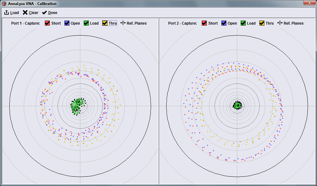
The toolbar on top allows you to
The main screen below the toolbar is split in two halves: The left side is for calibration where the signal output is port 1 (S11, S21), the right side is for calibration where the signal output is port 2 (S22, S12).
The charts show the current measurement and also the measurements that were already captured. Current reflective measurements (S11, S22) are black, current through measurements (S21, S12) are dark yellow. Note that the traces have a bit of a time lag because during calibration some extra filtering is active to reduce the noise.
Once a calibration standard is attached, you can press the appropriate button to capture the measurement. The captured measurement is then shown in the color that corresponds to the color on the button. A check mark in a button indicates that this measurement was already taken, but you can still take it again to replace the previous measurement. When you press the "Thru" button the software captures the measurements for S21 and S12 at the same time.
Once you are done, press the "Done" button and you will be prompted to save the calibration. Saving is optional.
Depending on what you want to measure you don't always need to perform a full calibration.
| To Measure | Calibrate |
|---|---|
| S11 | Short, Open, and Load on port 1. |
| S22 | Short, Open, and Load on port 2. |
| S21 | Thru on port 1. Load on port 1 improves accuracy with weak signals. |
| S12 | Thru on port 2. Load on port 2 improves accuracy with weak signals. |
| S11 and S22 | Short, Open, and Load on both ports. Thru calibration improves accuracy when the DUT has low insertion loss. |
If the calibration is incomplete the software still tries to come up with the best possible calibration coefficients given the available measurements. For example, calibrating with Open and Load on port 1 may still give you reasonable S11 measurements, especially near the center and the right half of the Smith chart.
Calibration standards for short and open circuit don't always terminate at exactly the same plane. To adjust for these differences you can click the "Ref. Planes" button and enter the adjustment values, either in millimeters (electrical length 1) or in picoseconds.

A positive number means that the calibration standard you are using is longer than the plane you want to calibrate at (Longer means that it terminates further away from the VNA). In the picture above the standard for open circuit is 1.2mm longer than the standard for short circuit. This is a good setting when using the calibration standards that come with the device.
1 Physical versus Electrical Length: Physical length is the actual length that you can measure with a ruler, while electrical length is the equivalent length if the speed of light was the same as in vacuum. The speed of light in cables and PCB traces is usually only around 2/3 of the speed of light in vacuum. If you have a trace with 1mm physical length the signal takes as long to traverse it as if it was 1.5mm of vacuum. That means the electrical length is 1.5mm.
Besides the full calibration described above it is also possible to perform a quick calibration to adjust the reference plane by pressing one of these buttons in the chart screen:

You can manually enter a distance by which to shift the reference plane and an additional signal loss. You can also terminate with either a short circuit or an open circuit and select the appropriate menu item to set the new reference plane to the position of the termination.
Note that this is not a substitute for a full calibration because it can't correct errors from the measurement setup. It is only accurate if no errors (discontinuities, mismatches) were introduced or removed compared to the full calibration.
This is the flow from measurement to the displayed trace:
When you open the matching circuit editor a new trace called "circuit" is created. You may have to configure the charts to show this trace.
The editor manages a sequence of circuit elements that can be added, removed, disabled, or rearranged.

Initially there are two elements: The first element is always the VNA (generator) and represents the point where the measurement is taken (the reference plane). The last element can be a static termination (open, short, 50 Ohms) or a complex load that is derived from a current measurement (S11, S22). With a static termination the matching circuit editor can also be useful in demo mode without an actual VNA (see example below).
The circuit editor then allows you to explore how things would change if you added components or transmission lines between the load and the VNA. The following components are available:
All components, except for series transmission lines, have no physical size. That means that they don't add any additional distance between the VNA and the load (they don't shift the reference plane), even though it may look that way in the user interface.
A series transmission line with positive length shifts the reference plane away from the load and towards the VNA (generator). A series transmission line can also have a negative length to shift the reference plane towards the load.
Individual circuit elements can be toggled on and off to easily observe the effect on the charts.
The example below shows how the circuit editor could be used to design a simple matching circuit for a detector diode. The diode is represented by the resistor with parasitic capacitance.


Here I am going to walk you through an antenna tuning procedure using a simple matching circuit. I started with this PCB that has an inverted F antenna on one side and room for some matching components (in a Pi configuration) on the other side:

I assumed that in the final application the PCB is mounted flush inside a plastic enclosure. In the setup I emulate that by taping the PCB to the outside of a plastic box.
This is the setup with the RF cable soldered to the board:

To perform a short-open-load calibration of the VNA I did the following:
Below is the calibration screen showing the raw readings. Blue is open, red is short, green is with load.

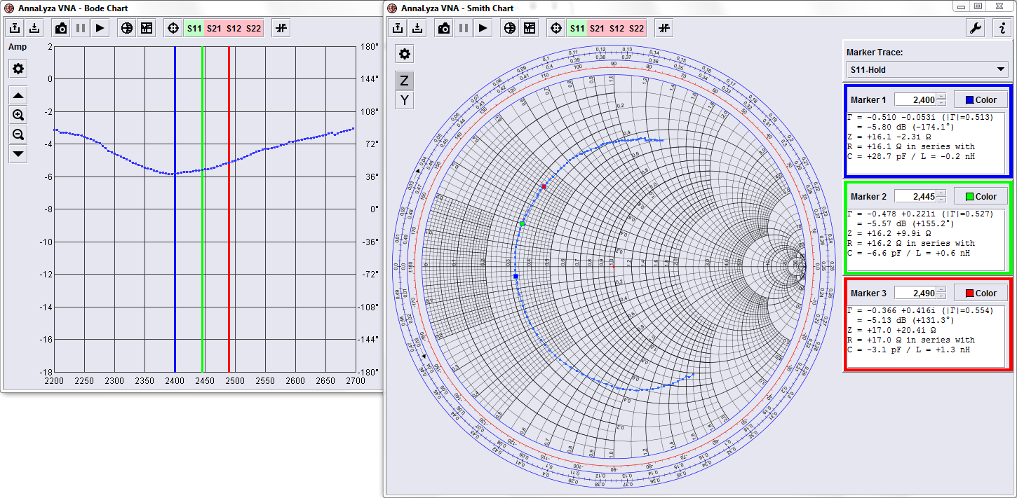
Then I removed the component again and shorted across C3 to measure the antenna without any matching elements.
Here is the result:
In real life you would probably first take a knife and copper tape and modify the antenna traces to improve the matching. That may not always be possible, and since I also wanted to evaluate the matching circuit editor I went straight to finding appropriate components.
I opened the matching circuit editor and played with different configurations and component values and I came up with this:

The parasitics are guesses based on the datasheets of the components. When the circuit editor is open I can see both the original S11 trace (in blue) and the simulated trace (in green). The simulated trace shows what would happen to the S11 trace if I had the matching circuit in place. The simulated trace updates in real time together with the S11 trace.
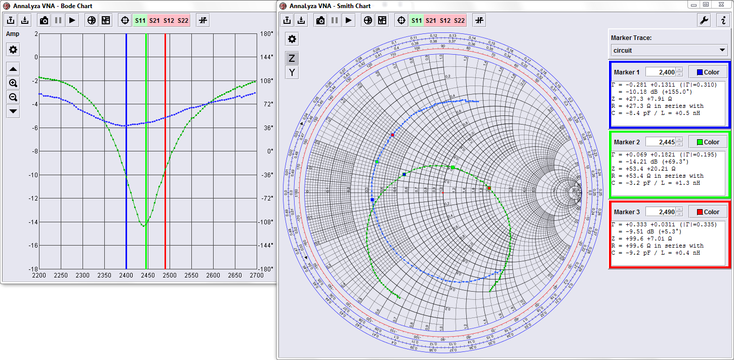
I took a snapshot of these traces so that I can compare them later with the actual measurement. Then I soldered the same component values that I used in the circuit editor to the PCB:

Finally, here is the real measurement (black trace) with the matching circuit in place:
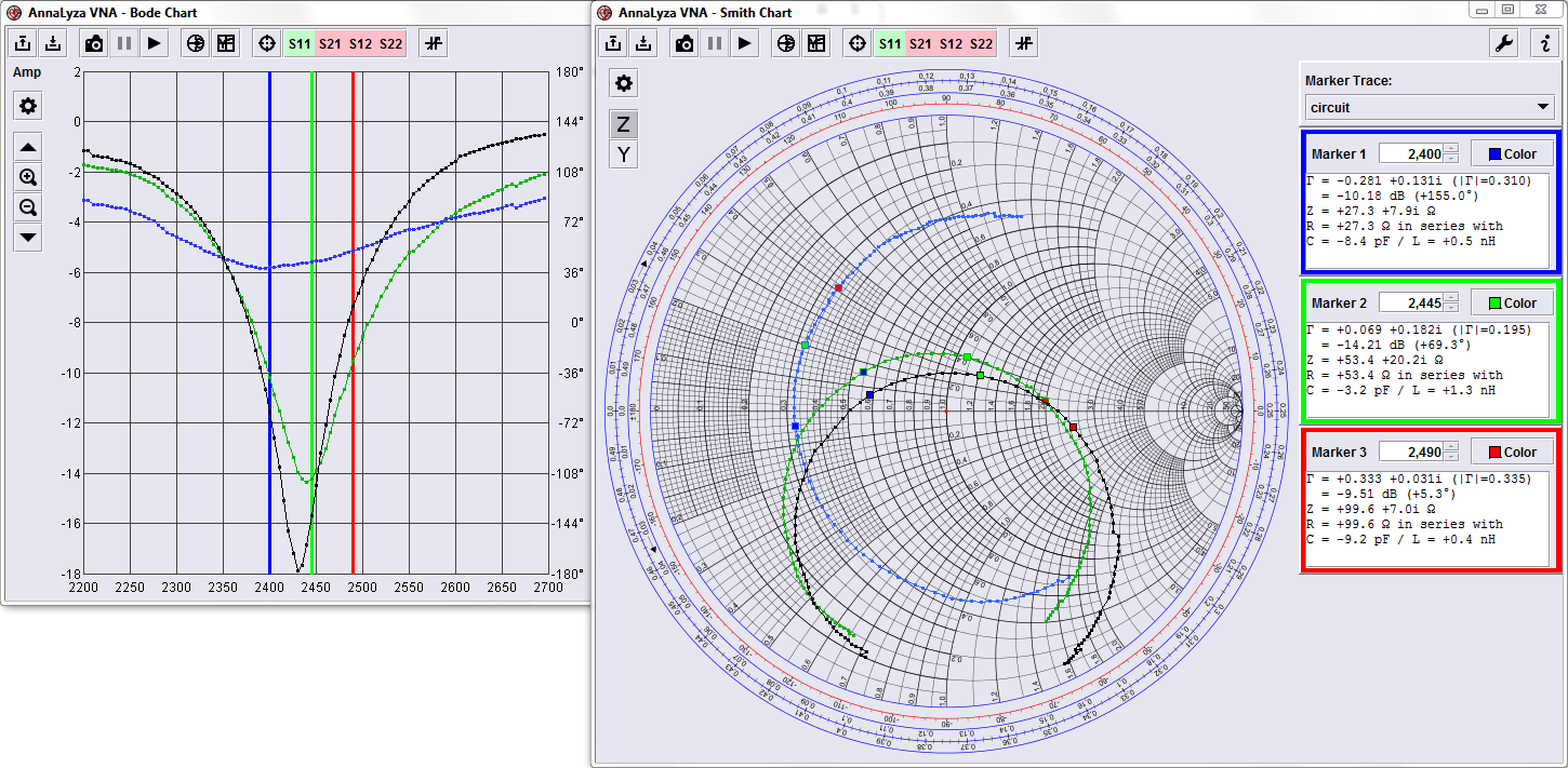
As you can see, the result is close to the prediction.
The discrepancies are probably due to a combination of a few factors: